Federal Reserve Economic Data

The FRED graph above compares job separations and hires in the U.S. economy.

Usually there are more hires than separations; that is, the number of employed people increases except during recessions. As we see in the graph, the recovery after the 2008-09 recession was remarkable in that hires were greater than separations in almost every month. Of course, this graph is dominated by the wild swings during the pandemic. So let’s look at the details of these separations.

The FRED graph below shows the proportions of three categories of separations: quits, layoffs, and others (retirements, for example). There are usually more quits that layoffs, except during recessions: With a weaker labor market, employees hesitate to quit while employers are more likely to fire some employees.

The pandemic has been no different, except that this pattern has been even stronger. It may appear that quits dropped off a lot, but the actual numbers of quits throughout the pandemic have actually been only a bit lower than usual. (Just hover your cursor over the graph to see the numbers).

How these graphs were created: For the first graph, search FRED for “separations” and select the seasonally adjusted series. From the “Edit Graph” panel, use the “Add Line” tab to search for and add “hires.” For the second graph, do the same, but searching for “quits,” “layoffs,” and “other separations.” From the “Format” tab, select graph type “Area” and stacking “Percent.”

Suggested by Christian Zimmermann.

The FRED Blog has discussed how stock market fluctuations don’t accurately reflect overall economic conditions in the U.S. Today, we throw real estate prices into the mix and see what patterns we can find.

The FRED graph above tracks total stock shares in blue and Case-Shiller national home prices in red during the most recent economic downturn. We use an index equal to 100 in the first quarter of 2020, the start of the COVID-19-induced recession, to help us easily compare these growth rates over time.

Real estate prices took off during the second half of 2020. Stock prices slumped during the first half of the year and did not quite catch up by the second half. (The same pattern is visible when comparing the Case-Shiller home price index to the Dow Jones Industrial Average.) But during the first quarter of 2021, stock prices grew steadily and ended up topping the year-to-year growth in home prices. If this were a game of rock-paper-scissors, paper (stocks) would have beaten rock (real estate).

Now let’s look at these same asset prices during the previous economic contraction—the Great Recession. In this graph, we see the slump in stock prices was deeper and lasted longer. Although home prices also declined, they did so much more gradually. In that round, the house of bricks (real estate) beat the house of cards (stocks).

How these graphs were created: Search for and select “Total Share Prices for All Shares for the United States.” From the “Edit Graph” menu, use the “Add Line” tab to search for “S&P/Case-Shiller U.S. National Home Price Index.” Again from the “Edit Graph” panel, select the “Edit Line 1” tab. In the “Units” drop-down menu, select “Index (Scale value to 100 for chosen date)” and choose “2020-02-01” for the first graph and “2007-12-01” for the second graph. Adjust the date range to mirror the dates shown in the blog post.

Suggested by Diego Mendez-Carbajo.

The World Bank has many data series that allow comparisons among countries over time, and today’s FRED graph reveals some trends in life expectancy and national income.

Lower life expectancy in low-income countries has been catching up. In 1982, life expectancy at birth in low-income countries was about 66% of what it was in high-income countries. Then life expectancy increased at a faster pace in low-income countries, and the value rose to 78% by 2018. This rising longevity, especially in relation to longevity in high-income countries, is remarkable because it doesn’t coincide with an improvement in relative economic performance.

In 1982, real GDP per capita in poor countries was 2.8% of what it was in rich countries. In 2018, it was 1.8%. Despite poor countries losing ground to rich countries on the economic front (GDP per capita), they gained ground on the health front (life expectancy at birth).

For more information, read on… Countries in this analysis are classified as low income or high income depending on their 2019 gross national product per capita. And countries aren’t always in the same group from one year to the next, of course.

1. This variability doesn’t affect the conclusion here that there’s a disconnect between economic performances and life expectancy.
2. This general conclusion from the FRED graph also holds for individual countries. For example, life expectancy in Benin grew from 63% of life expectancy in the U.S. in 1980 to 70% in 2018. But Benin’s GDP per capita remained below 1% of U.S. GDP per capita for that period.
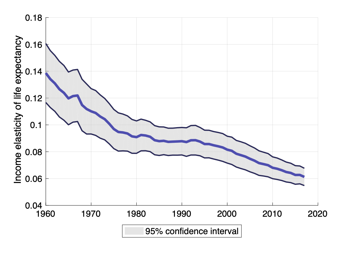
3. Finally, the statistical correlation of life expectancy and GDP per capita across individual countries has been steadily declining since the 1960s, shown in the graph below. The FRED graph above is a manifestation of this decline.

How this graph was made: Search for and select “Life Expectancy at Birth, Total for Low income Countries.” From the “Edit Graph” panel, use the “Customize data” search field to search for and add the series “Life Expectancy at Birth, Total for High Income Countries” to the same line. In the formula bar, type a/b*100. Next, under the “Add Line” tab, search for and add “Constant GDP per capita for Low Income Countries” and “Constant GDP per capita for High Income Countries.” In the formula bar, type a/b*100.

Suggested by Guillaume Vandenbroucke.