March | 2020 | FRED Blog

Calculating the value of women’s unpaid work

U.S. women's unpaid labor basically equals the state GDP of New York

Posted on March 9, 2020

Yesterday was International Women’s Day, so FRED is taking the opportunity to examine one economic contribution from women that’s often ignored: The value of women’s domestic labor that goes unpaid.

For this calculation, we use Oxfam’s methodology: We calculate the total amount of hours that women spend doing unpaid household work and then use the minimum wage to put a dollar value on that work:

Take the number of women above age 16 and multiply by 26.7 hours, which is, according to the Bureau of Labor Statistics, the average number of hours per week women spend on unpaid household work.
Multiply this weekly value by 52, the number of weeks in a year.
Multiply the result by the federal minimum wage.
Divide this annual dollar amount by the consumer price index to adjust for inflation. (Note we use annual data here, aggregated at the end of each year, to make the graph easier to read.)

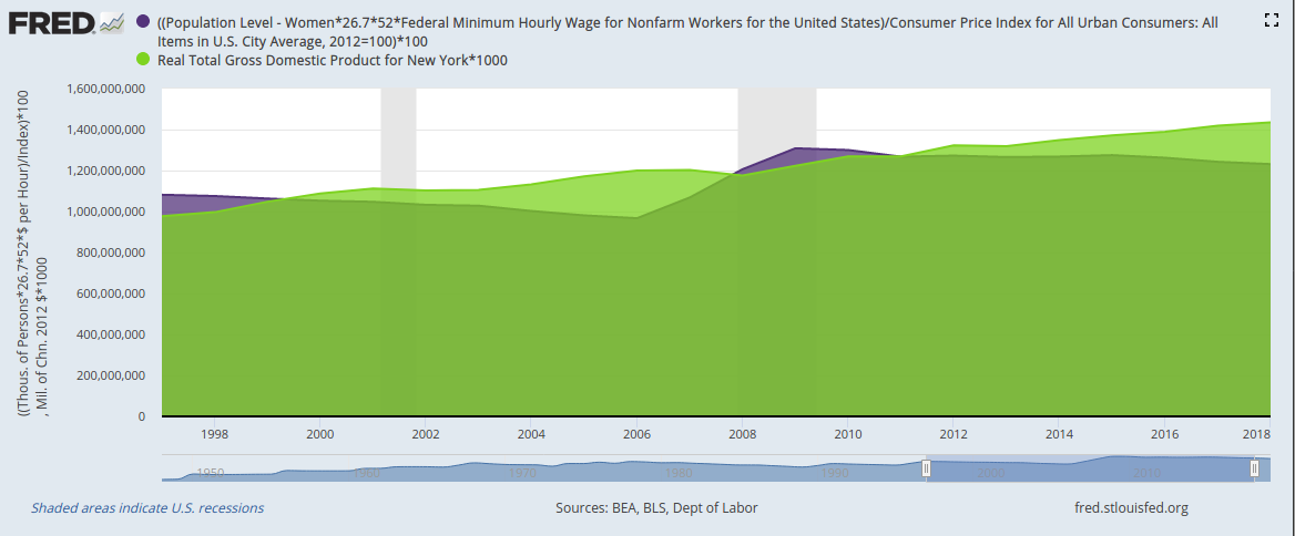
OK. Nice graph. But how big a number is this? To put it in context, let’s compare the value of women’s unpaid labor with all the economic activity recorded in the state of New York.

Customize | Download data

For 2018 (the most recent data available), the dollar value of women’s unpaid work in the U.S. was equal to 86% of all the economic activity recorded in the state of New York. In other years—say, the late 1990s and late 2000s—the value of women’s unpaid work even surpassed New York state GDP. And keep in mind this value is at the low end of the possible range because we use the federal minimum wage and not, for example, higher state minimum wages let alone market wages that correspond to the specific work being done.

How these graphs were created: For the first graph: Search for and select the population of women (series ID LNU00000002). From the “Edit Graph” panel, use “Edit Line”/”Customize data” to search for and add the series for the federal minimum wage (series ID FEDMINNFRWG) and CPI (series ID CPIAUCSL). Adjust frequency to annual. Apply formula ((a*26.7*52*b)/c)*100. From the “Format” tab, choose graph type “Area” and change the color to International Women’s Day purple. For the second graph: Start with the first graph. From the “Edit Graph” panel, adjust the units for CPI to 100 in 2012. Then use the “Add Line” tab to search for and select New York state GDP (series ID NYRGSP). Apply formula a*1000. Finally, adjust the sample period to a time when both series are available.

Suggested by Diego Mendez-Carbajo.

View on FRED, series used in this post: CPIAUCSL, FEDMINNFRWG, LNU00000002

The economic impact of a pandemic

Wages during the Spanish Influenza

Posted on March 5, 2020

How does a pandemic affect an economy? Obviously, it’s a multilayered topic and FRED has limits to what it can reveal. The good news, of course, is that large-scale pandemics are rare. So the economic effects for most of these outbreaks are hard to see by graphing data. But we can take two of the most extreme examples, which will have visible effects in the data: the Black Death of the mid 14th century and the Spanish flu of 1918-1920.

We already covered the first one in a post from December 2018. So we look at the second one today: the influenza outbreak of 1918, commonly known as the Spanish flu. According to the Centers for Disease Control and Prevention, this pandemic infected about a third of the world’s population and killed at least 50 million people.

So, what economic effects can we see? The graph above shows hourly wages for various trades in the United States, and one particular feature of the data is a run-up of wages from 1918 to 1920 (followed by a drop, with the recession of 1921). This effect is consistent with the economic theory behind a sudden loss of population, just as we showed for the Black Death.

In the case of the Spanish flu, we also need to disentangle it from the consequences of World War I. Luckily, there’s some additional analysis in a St. Louis Fed Review article and other work by Thomas Garrett. Indeed, not all U.S. cities were affected in the same way by the Spanish flu or by WWI casualties. Exploring these differences, Garrett shows that the effect of the Spanish flu on wages was real and even bigger than the effects of WWI.

How this graph was created: Search for “Average Hourly Money Earnings” and click on one of the relevant series. From the “Edit Graph” panel, open the “Add Line” tab and search for more series. Repeat as needed.

Suggested by Christian Zimmermann.

View on FRED, series used in this post: A08052USA052NNBR, A08053USA052NNBR, A0850AUSA052NNBR, A0851AUSA052NNBR, A0854AUSA052NNBR

Does the local economy influence voters?

A look at state median household income growth

Posted on March 2, 2020

The health of our local economy affects our outlook, which in turn can affect our decisionmaking, including how we cast our votes. Some classic research shows the economy is an important factor in national elections; and some newer research specifically links disposable income and military casualties to election results.

FRED has data to help you traverse the economic landscape during elections. This map shows the growth rate of median U.S. household income state by state.

Median is defined as the value at which half the households are above and half below. In a majority election, for example, the median voter would be the determining factor. We look at households here, which obviously could include several voters.
We transformed the raw data on household income to a growth rate, to show how things have changed from the previous year. (By the way, these data are nominal and, thus, include general inflation.)

The darker the color, the more growth—and, in simplified terms, the likelier it is an incumbent politician will be re-elected. Now, at the time of posting, the latest data we have is for 2018. To see how incomes grew for previous years, click on the View in GeoFRED link to get to all the mapping tools: The legend box has arrows that let you move from year to year, all the way back to 1990, which includes seven U.S. presidential elections.

How this map was created: The original post referenced an interactive map from our now discontinued GeoFRED site. The revised post provides a replacement map from FRED’s new mapping tool. To create FRED maps, go to the data series page in question and look for the green “VIEW MAP” button at the top right of the graph. See this post for instructions to edit a FRED map. Only series with a green map button can be mapped.