Federal Reserve Economic Data

Economic research has found that the neighborhood in which a child grows up can influence their adult outcomes,  such as educational attainment and income. That alone is a powerful enough reason for US households to pack up and move across the city or even around the country.

Every year, the US Census tracks movement (and other data) throughout the country by surveying a broad sample of households and records: Among other information, they track their current and previous counties of residence. With those data, the Census calculates a 5-year estimate of the difference between inflows and outflows of residents from  county to county. This is called net migration.

The FRED map above shows the estimated county-to-county net migration flows between the years 2016 and 2020. We customized the data groupings to sort all 3,140 US counties into two groups: counties that gained residents and thus registered positive net migration (shown in green) and counties that lost residents and thus registered negative net migration (shown in yellow). No clear pattern is visible to the naked eye, so we created a second data visualization to group the counties by state.

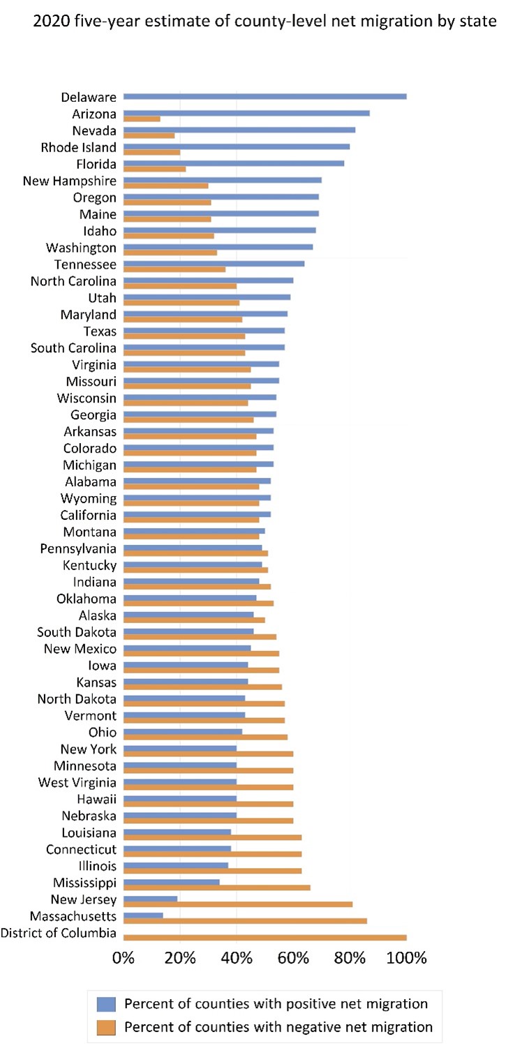
The second graph shows the percent of counties in each of the 50 states plus the District of Columbia that recorded positive net migration (blue bars) and the percent of counties in each state that recorded negative net migration (orange bars). The states are sorted from largest to smallest proportion of counties with net resident inflows. Keep in mind that different states have different numbers of counties. Note that all three counties in Delaware recorded positive net migration, so that state is listed at the top. Conversely, the District of Columbia is a county equivalent and, because it experienced negative net migration, it’s listed at the bottom.

Overall, the bar graph shows states such as Arizona, Nevada, and Florida had far more counties recording net resident inflows than outflows. The data do not show where the new residents came from or their demographic characteristics. We can’t say if those states gained residents from states such as Massachusetts, New Jersey, and Illinois, which lost residents. Finally, there are 4 states where the percent counts of counties is slightly off: Each of these states is home to one county that experienced zero net migration. You can see those counties, highlighted in red, in this FRED map.

How this map was created: In FRED, search for “Net County-to-County Migration Flow (5-year estimate) for Miami-Dade County, FL.” Click on “View Map.” To change the data groupings, use the “Data grouped by” dropdown menu to select “User Defined Method.” Change the “Number of color groups” to 2 and enter “0” in the topmost box.

Suggested by Diego Mendez-Carbajo.

The graph above shows how Treasury security holdings by the banking sector and the Treasury yield have evolved over the past five years. The red line shows the Treasury and agency securities that commercial banks hold as a share of their total assets since mid-2018. The green line shows the market yield on 10-year Treasury securities over the same period.

This relationship between market yields and bank holdings seems to be divided into three distinct phases:

1. In the period before the pandemic-related recession, which began in February 2020, these lines seem to have a slight inverse relationship: Treasury holdings trended up while the Treasury yield declined.
2. In the two years after the recession began, both lines increased together after a brief initial dip.
3. In the past year, nearly three years since the pandemic recession ended, the inverse relationship reappears, with Treasury holdings trending down and Treasury yields increasing.

One can understand these three phases as an interplay between demand and supply.

Before the pandemic, banks were demanding more Treasuries for their portfolio, and the increase in demand pushed up the price of Treasuries, which in turn depressed the yields. As a result, we see that the red line rose slightly as the green line fell slightly.

During the pandemic, a large amount of Treasury debt was issued to finance the stimulus and spending during the crisis. The issuance of Treasury debt is a large supply shock to the Treasury market. As opposed to the previous period when Treasury demand was driving the yields, there was more Treasury debt than banks (and other potential buyers) were willing to hold at the original price. As a result, the price of Treasury debt went down and the yields rose to entice the banks and other buyers to increase their holdings.

This trend held for nearly two years after the pandemic recession, until demand forces took hold again. In this most-recent period, demand for Treasuries has slowed, which has resulted in lower prices for securities and a faster increase in yields than before.

How this graph was created: Search FRED for “All Commercial Banks Total Assets” and select “Total Assets, All Commercial Banks.” Use the “Edit Graph” button in the upper right corner to open the editing box. Scroll down to “Customize data.” In the text box, search for “Treasury and Agency Securities” and select “Treasury and Agency Securities, All Commercial Banks.” Select “Add” next to the text box. Below this section in “Formula,” enter b/a and select “Apply.” Next, click the gray “ADD LINE” box at the top. In the search box, search for “Market Yield on U.S. Treasury Securities” and select “Market Yield on U.S. Treasury Securities at 1-Year Constant Maturity, Quoted on an Investment Basis.” Below this section in “Formula,” enter a/100 and select “Apply.”

Suggested by Jessie LaBelle and Yu-Ting Chiang.

The FRED Blog has used data from the US Census to discuss income inequality and racial housing patterns across the US at the county level. Today, we tap into those datasets again to highlight two different city-level extremes of economic inequality.

The FRED graph above shows Census data on the racial dissimilarity index (solid lines) and income inequality (dashed lines) in two locations: Miami-Dade County, Florida (in orange), and Lackawanna County, Pennsylvania (in purple).

Why those two counties? Because they’re home to Miami and Scranton, one of the most and one of the least income-segregated large US cities, respectively.

Recent research from Hannah Rubinton and Maggie Isaacson at the St Louis Fed examines the relationship between income inequality and income segregation in the 100 largest US cities: Their calculations show that, in 2015, Miami was the 3rd most-unequal in income distribution and in the top 25% of most-income-segregated cities. Scranton, on the other end, was 3rd least-unequal in income distribution and 4th least-income-segregated of all 100 cities.

For more about this and other research, visit the website of the Research Division of the Federal Reserve Bank of St Louis, which offers an array of economic analysis and expertise provided by our staff.

A little bit more about the analysis from Rubinton and Isaacson: They find that cities with higher levels of income inequality have higher levels of income segregation. They use neighborhood-level Census data for each city and measure income inequality using the Gini coefficient. This coefficient ranges between 0 and 1, where larger values indicate a more-unequal distribution of income within a city. They measure income segregation by comparing the distribution of income in each neighborhood to the overall distribution of income in the city. They calculate an index that ranges between 0 and 1, where larger values indicate it’s more common for different income groups to live in different areas of a city.

How this graph was created: Search FRED for “White to Non-White Racial Dissimilarity (5-year estimate) Index for Miami-Dade County, FL.” Next, click the “Edit Graph” button, select the “Add Line” panel, and search for the same series for Lackawanna County, PA. Repeat the “Add Line” step to add both the “Income Inequality” series in Miami-Dade County and in Lackawanna County to the graph. Last, use the “Format” panel to change the Y-axis position of the income inequality series and to customize the color and format of the lines.

Suggested by Diego Mendez-Carbajo.